Hemispheric Image Processing in R

Introduction

This part of the guide will focus on hemispheric image processing in R, and ImageJ software packages.

Copy the code below into R studio, make sure the working directory is set correctly on line 18 and that you have the correct file path pointing to your installation of Ghost Script on line 10.

R code for hemispheric photo analysis:

# This uses the local area thresholding from imagerExtra
# Needs ghostscript installed on PC
# Load packages
require(imager)
require(imagerExtra)
require(lubridate) 
require(compiler)

# Set location of ghostscript executable (only needs to be done once)
Sys.setenv(R_GSCMD="C:/Program Files/gs/gs9.55.0/bin/gswin64c.exe") 

# Note, the following should be in the directory (along with the .jpg files)
# LAICAM.exe
# call-GFA.bat
# GFA-WIN.exe

# Set working directory
setwd("U:/RPI Project/Working Directory")



# List files
allPics <- list.files(pattern = ".jpg")
# allPics<- list.files(pattern = "-07|-09|-12|-16")

# Define function to rotate, pad and greyscale using imager
rotate_imgs <- function(allPics, x) {
  for(x in seq_along(allPics)) {
    filename <- allPics[x]
  blueChan <- B(load.image(allPics[x]))
  wind201 <- ThresholdAdaptive(blueChan, 0, range = c(0,1), windowsize = 201)
  wind17 <- ThresholdAdaptive(blueChan, 0, range = c(0,1), windowsize = 17)
  comb <- threshold((wind17 + wind201), 1) 
  rotImg <- imrotate(comb, 3) 
  bitmap(file=paste("out_",substring(filename, 1, 10),".", substring(filename, 12,17), ".bmp", sep =    ""), width=4147, height=3888, units="px", type = "bmpmono")
  plot(rotImg, axes = F)
  dev.off()
}
}

# Use function to produce output
start.time <- Sys.time()
rotate_imgs((allPics[1:5000]))
end.time <- Sys.time()
end.time - start.time
# Note  - it is necessary to convert the .bmp images to 8-bit using ImageJ at the point #

### GFA (gap fraction analysis)
# write batch script
bmp.list <- list.files(pattern = ".bmp")
batch.list <- paste("call call-GFA.bat", substring(bmp.list, 1, 21), "c", sep=" ")
write.table(batch.list, file = "batch.bat", row.names = F, col.names = F, quote = F)

# run batch files
shell("batch.bat")

### LAICAM (leaf area index) - make sure parameter.txt file is not in the directory
# write batch script

txt.list <- list.files(pattern = ".txt")
batch.list.txt <- paste("LAICAM parameter.txt", txt.list, "gf_result_file.txt", sep=" ")
write.table(batch.list.txt, file = "processing_list.bat", row.names = F, col.names = F, quote = F)

# Write parameter.txt file
params <- c("0", "0", "0", "0", "0", "0.0", "0.0", "0.0", "0.0", "1") 
# see laicam.pdf for explanation of these parameters

write.table(params, file = "parameter.txt", row.names = F, col.names = F, quote = F)

# run batch file
shell("processing_list.bat")

# Read results
gf_heads <- c("Progr.Name","Data.file.name", "Slope", "Aspect", "Ref", "Z_ann", "H_ann","LeafR", "LeafT",	"SoilR", "Lsat", "EC", "EG", "ST", "CI.LX", "SO", "CO", "CC", "Le", "X", "Err","A", "Lsl","Lsh","Ke","Kb.i","FC","FS")
              gf_results <- read.table("gf_result_file.txt", header = F, col.names = gf_heads)
              
              # End

Copy hemispheric images into your working directory

Copy the photos from your raspberry pi camera into your working directory. If you haven’t taken any photos yet and simply want some examples you can download some exemplar photos here.

Do a visual check of your photos and remove any that are unlikely to give good results. Oversaturation and issues with moisture early in the morning are likely to impair the quality of your photos.

Rotating, padding and making photos greyscale .bmp

The photos need to be rotated so that the top of the image faces north. This is set on line 34 where the number indicates the number of degrees necessary to rotate the image. In my case a three-degree rotation was required, alter this to suit your photos.

Select the code from lines 1 – 45 and in the top right corner of R studio press ‘run’. If everything has run correctly you will end up with photos looking like this:

Converting photos with ImageJ

At this point go into the working directory and delete all the .jpg photos, so you are only left with your converted .bmp images (it will make the next step quicker).

Getting your coordinates from ImageJ

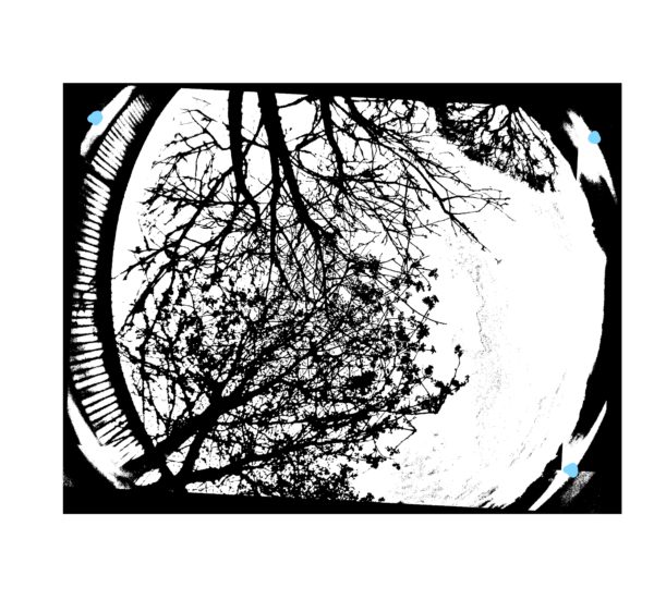
Three XY coordinates are needed from the horizon of the greyscale photos. Open ImageJ and open one of the converted photos, by selecting ‘File’ then ‘Open’.

After the photo has opened hover your mouse over a point on the horizon and take a note of the coordinates. Take three coordinates from the horizon using a roughly triangular method. The blue dots on the photo below indicate good points to take coordinates from. This is only required for one photo. The coordinates will be added to our call-GFA.bat in a later step, so keep a note of them.

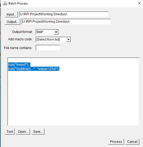
Batch inverting and converting to 8-bit .bmp in ImageJ

The gap fraction analysis that will run in R needs to be able to tell the difference between the background and foreground. To do this the image must be inverted and converted to 8-bit.

In ImageJ select ‘Process’ – ‘Batch’ – ‘Macro’. Make sure that your input and output directory is set to your working directory, and make sure that the ‘output format’ is ‘BMP’. After that add the code below into the box at the bottom.

run("Invert");
run("Subtract...", "value=254");

It should look like this:

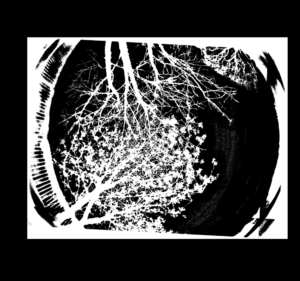
Press ‘Process’ and let ImageJ convert all the images. Once done, the photos should look like the one below and be of an equal file size.

Editing call-GFA.bat

In an earlier part of this tutorial, call-GFA.bat was created in the working directory. Right-click on it and click ‘Edit’. Copy the code below into the file. Alternatively, you can download my copy of call-GFA.bat here.

@echo off
if %1.==.goto usage
for %%i in (1,2) do (
if exist %1 (
echo %1 > temp
goto suite )
if exist %1.bmp echo %1.bmp > temp
if not exist %1 if not exist %1.bmp goto filenotfound
:suite
echo 1 >> temp
echo 648 688 >> temp
echo 568 2924 >> temp
echo 3776 888 >> temp
echo %2 >> temp
if %2==g (
echo %3 >> temp )
if %%i==1 (
echo y >> temp
echo 10.0 >> temp
echo 65.0 >> temp
echo 1.0 >> temp )
if %%i==2 (
echo n >> temp
echo 18 24 >> temp
echo 1.34 >> temp )
GFA-WIN < temp
)

if exist gf_%1.txt (
del gf_%1.txt )
if exist gs_%1.txt (
del gs_%1.txt )
ren gapfract.txt gf_%1.txt
ren gapsize.dat gs_%1.txt

goto end
del temp
:usage
echo USAGE : call-GFA <file_name> <c/g> <if g, threshold_value>
goto end

:filenotfound
echo file not found
goto end

:end

The key elements that require editing are lines 11 to 13 which require the input of your photo coordinates from ImageJ. Line 25 sets the magnetic declination, the magnetic declination of a particular location can be looked up online.

Line 24 sets your zenith and azimuth sectors, the number of sectors I have selected is ‘industry standard’ but you can change them to suit your needs if you like.

call-GFA.bat will spit out both gap fraction and gap size results. It is the gap fraction results that we are most interested in.

After editing, save the changes and exit the file.

Running the gap fraction analysis.

It’s now time to run the gap fraction analysis. Select the R code from line 48 to the bottom and in the top right of R studio press ‘run’.

If there are a lot of photos to analyze this will take some time.

Reading your data into Excel

After the analysis has run a ‘gf_results.txt’ file will be produced. To open this in a readable format the import text/CSV function of Excel can be used.

When the file has been loaded in you will notice that the columns are not named. The column names can be found in lines 74 -75 of the R code, for a detailed explanation of these readouts you can refer to the laicam pdf which is in the ‘MANUALSTRUC.zip’ download available here.

Column 18 has the data we are most interested in which is the fraction canopy closure (CC).

For ease of use, it might be worth changing the date-time into an Excel readable format. To do this select a blank column and enter the formula below where ‘B2’ is the column with the results file name. You can then format the column with a custom format. Use: dd/mm/yyyy hh:mm:ss this will give you a nice column that describes the date and time that your photo was taken.

=SUBSTITUTE(MID(B2,8,10),".","-")+ REPLACE(REPLACE(MID(B2,19,6),5,0,":"),3,0,":")

Statistics

For ease of use, I copied my data into Minitab to have a brief look at it and see if there was a trend. I am aware that many people won’t have access to Minitab, so when I have a couple more weeks’ worth of data I will do some analysis of it in R, and post the results.